
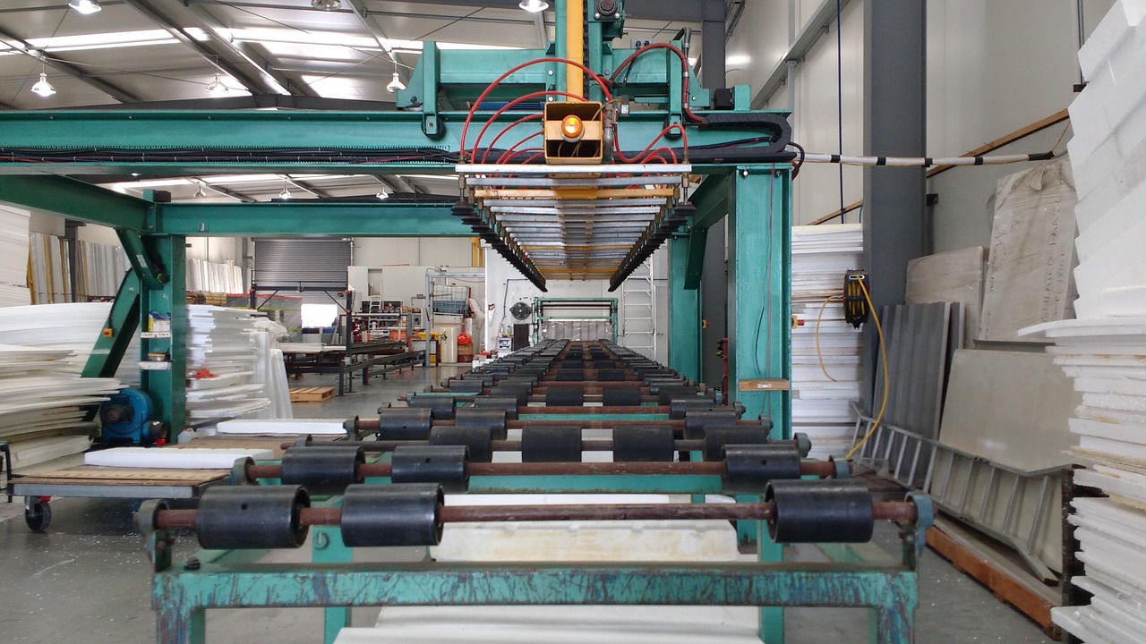



Capacity utilisation is the share of a plant’s possible output that a company actually produced in a period. Read it next to quarterly results and a lot of puzzling numbers start to make sense: why a cement maker’s margin jumped while sales grew only modestly, or why a company that just opened a shiny new line reported weaker profitability than the quarter before.
We look at it as the bridge between the sales line and the margin line. Sales tell you how much was sold. Utilisation tells you how hard the fixed assets worked to get there, and that is what decides how much of the revenue survives as operating profit.
In this article
- What capacity utilisation actually measures
- Why capacity utilisation moves margins before sales
- A worked example: one plant, three quarters
- Where to find capacity utilisation numbers
- The economy-wide reading: RBI’s OBICUS survey
- How we use capacity utilisation when reading results
- Common mistakes with capacity utilisation
What capacity utilisation actually measures
The formula is simple. As Investopedia puts it, you divide actual output by potential output and multiply by 100. A factory that can make 1,000 units a day and makes 800 is running at 80%.
The tricky word is “potential”. Wikipedia’s entry on capacity utilization describes two ways of defining it:
- Engineering (technical) capacity: the most a plant can produce in the short run with its existing equipment. This is the “nameplate” figure companies usually quote, such as tonnes per annum for cement or steel.
- Economic capacity: the output level beyond which average cost starts to rise. The same entry notes that this measure typically comes out around 10 percentage points higher than the engineering measure, though both move the same way over time.
Why does this matter to an investor? Because two companies quoting “85% utilisation” may not be using the same denominator. One may count nameplate capacity, another may count capacity under normal shifts. When a company switches definitions between presentations, the trend can look better than it is. Always check the footnote.
Why capacity utilisation moves margins before sales
A manufacturing plant carries a chunk of costs that barely change with output: employee costs at the plant, maintenance contracts, insurance, a base level of power, and depreciation on the machines. Investopedia’s explanation of low utilisation makes the point directly: fixed costs get spread over fewer units, which pushes up the cost per unit and can squeeze profit margins.
Run that logic in reverse and you get the reason margins often jump before sales look exciting. Every extra tonne pushed through an underused plant carries only its variable cost. The fixed cost has already been paid. So when utilisation climbs from, say, the mid-60s to the low-80s, EBITDA can grow at several times the pace of revenue. This is the same mechanism we covered in operating leverage in quarterly results, seen from the factory floor.
Revenue tells you what was sold. Utilisation tells you how much of the fixed cost base got paid for along the way.
A worked example: one plant, three quarters
The numbers below are hypothetical and chosen only to show the arithmetic. They do not describe any listed company.
Picture a cement company with one plant that can produce 10 lakh tonnes a quarter. It sells at ₹5,000 a tonne, variable cost (fuel, power, raw material, freight) is ₹3,200 a tonne, and fixed costs are ₹80 crore a quarter.
| Item | Quarter A | Quarter B | Quarter C (new line added) |
|---|---|---|---|
| Capacity in the quarter (lakh tonnes) | 10.0 | 10.0 | 12.5 |
| Production and sales (lakh tonnes) | 6.5 | 8.0 | 8.5 |
| Capacity utilisation | 65.0% | 80.0% | 68.0% |
| Revenue (₹ crore) | 325 | 400 | 425 |
| Variable cost (₹ crore) | 208 | 256 | 272 |
| Fixed cost (₹ crore) | 80 | 80 | 100 |
| EBITDA (₹ crore) | 37 | 64 | 53 |
| EBITDA margin | 11.4% | 16.0% | 12.5% |
| Fixed cost per tonne (₹) | 1,231 | 1,000 | 1,176 |
Quarter A to Quarter B: the margin leaps
Volumes rise from 6.5 to 8.0 lakh tonnes. Revenue goes up about 23%, from ₹325 crore to ₹400 crore. EBITDA, though, goes from ₹37 crore to ₹64 crore, a rise of roughly 73%. The margin expands from 11.4% to 16.0% without any change in price or in cost per tonne of fuel.
All of that extra margin comes from one line in the table: fixed cost per tonne falling from ₹1,231 to ₹1,000. Nothing clever happened. The plant simply worked harder.
Quarter B to Quarter C: sales up, margin down
Now the company commissions a new line that adds 2.5 lakh tonnes of quarterly capacity, and fixed costs rise to ₹100 crore to run it. Demand grows, but only to 8.5 lakh tonnes. Revenue rises about 6% to ₹425 crore. A headline writer might call it a decent quarter.
Look one level down, though. Utilisation falls from 80% to 68% because the denominator grew faster than output. Fixed cost per tonne climbs back to ₹1,176. EBITDA drops about 17% to ₹53 crore and the margin slips to 12.5%. Sales up, profit down. If you read only the revenue line you would miss the whole story.
This is the pattern to expect in the first few quarters after a big expansion in steel, cement, chemicals or autos. The capacity arrives in one go; demand fills it gradually.
The mid-quarter commissioning wrinkle
Suppose the new line in Quarter C started only halfway through. Then it was available for half the quarter, so effective capacity was 10 + 1.25 = 11.25 lakh tonnes, not 12.5. Utilisation on that basis is about 75.6%, not 68%. Companies differ on whether they quote utilisation on full nameplate capacity or on time-weighted effective capacity. Neither is wrong, but you need to know which one you are comparing.
Where to find capacity utilisation numbers
Indian companies do not have to report utilisation in a standard format, so the data is scattered. These are the usual places:
- Investor presentations: cement, steel, auto and chemical companies often show capacity and production, or utilisation directly, in their quarterly decks.
- Earnings calls: analysts ask about it constantly. Our guide to reading an earnings call transcript covers how to check management’s comments against the reported numbers.
- Annual reports: the management discussion section frequently lists installed capacity and actual production by product.
- Derived numbers: where a company gives volumes and capacity but not utilisation, divide one by the other yourself, adjusting capacity for the length of the period.
For services businesses the idea carries over under other names. IT firms talk about utilisation of billable staff, hotels about occupancy, airlines about load factor. The metric changes; the logic of spreading a fixed base over more output does not.
The economy-wide reading: RBI’s OBICUS survey
At the level of the whole manufacturing sector, the Reserve Bank of India runs the Order Books, Inventories and Capacity Utilisation Survey, known as OBICUS. In its October 9, 2026 release launching the 75th round, the RBI says it has run the survey quarterly since 2008, that it collects item-wise production against installed capacity among other data, and that the survey feeds into monetary policy formulation.
The latest results, released on October 7, 2026, cover April to June 2026 (Q1 of FY2026-27). The survey covered 1,076 manufacturing companies, and 994 of them responded on capacity utilisation. Here is what the RBI’s Table 1 shows for the last five quarters:
| Quarter | Capacity utilisation (%) | Seasonally adjusted (%) |
|---|---|---|
| Q1 FY2025-26 | 74.1 | 75.8 |
| Q2 FY2025-26 | 74.3 | 74.8 |
| Q3 FY2025-26 | 75.6 | 75.5 |
| Q4 FY2025-26 | 77.4 | 75.2 |
| Q1 FY2026-27 | 74.6 | 76.3 |
Notice what happened between the last two rows. Raw utilisation fell from 77.4% to 74.6%, which looks like a slowdown. Yet the seasonally adjusted figure rose by 110 basis points to 76.3%. The gap between the two series tells you why: in January-March the raw number sat above the adjusted one, and in April-June it sat below it, which means the RBI’s model treats the first as a seasonally strong quarter and the second as a seasonally weak one. Most of the raw drop was the calendar. Compared with the same quarter a year earlier, the RBI says both the raw and seasonally adjusted numbers were up 50 basis points. The RBI calculates the adjusted series with X13-ARIMA-SEATS, treating the Covid lockdown quarter of April-June 2020 as an outlier.
The same release shows new orders growing 3.7% quarter on quarter and 14.3% year on year in Q1 FY2026-27, against 2.9% and 4.0% in the previous quarter (these growth rates are for a common set of companies that responded across three rounds). Finished goods inventory rose to 23.9% of sales from 21.0%, and raw material inventory to 25.5% from 23.9%.
The lesson for reading company results is the same one the RBI table teaches: compare a quarter with the same quarter last year, or use seasonally adjusted data, before calling a trend. A cement company’s April-June utilisation will often look worse than January-March for reasons that have nothing to do with competitiveness.
How we use capacity utilisation when reading results
- Pair it with fixed cost per unit. If utilisation rose but margins didn’t, something else ate the gain: a price cut, higher fuel costs, or a one-off. Find it.
- Check the denominator after expansions. A dip in utilisation right after new capacity arrives is normal. A dip that persists for several quarters says demand isn’t showing up.
- Watch the capex trigger. When a sector runs hot for a while, companies tend to announce new plants. That fresh supply can later pull utilisation, and pricing power, back down.
- Look at asset efficiency together. Utilisation explains a lot of the movement in fixed asset turnover, since both measure how much the plant is producing for the money sunk into it.
- Read the inventory line. High production with rising finished goods inventory can mean a company is running plants hard to keep unit costs low while stock piles up unsold. Utilisation looks good; cash flow does not.
Common mistakes with capacity utilisation
The first is treating 100% as the goal. Plants need downtime for maintenance, and pushing near the physical limit often means overtime and extra shifts that raise unit costs. That is exactly why economists use the economic definition alongside the engineering one.
The second is comparing utilisation across sectors. A refinery, a cement kiln and a garment unit run at structurally different levels. Compare a company with its own history and with direct peers.
The third is ignoring product mix. A plant running at 90% on low-margin grades can earn less than one at 75% on premium products. Utilisation explains cost absorption; it does not tell you what the plant is making.
For the full checklist that this metric plugs into, our pillar guide on how to analyse quarterly results of a company walks through revenue, margins, other income and cash flow in order.
Disclaimer: This article is for educational purposes only and is not investment advice. The worked example uses hypothetical numbers. Please do your own research or consult a SEBI-registered adviser before making investment decisions.

Leave a Reply
Join the conversation
Commenting is open to registered readers. Sign up with just your email — no password needed, and it takes under a minute.
Sign up to comment Log in